November 17, 2021
The interpretation of faults in 3D seismic data is a critical component of hydrocarbon exploration and development workflows. Faults frequently control factors such as reservoir compartmentalization and fluid migration and may create drilling hazards. A comprehensive understanding of faulting is a prerequisite for the safe and efficient development of the subsurface. By leveraging the latest technologies such as cloud computing and machine learning, Landmark has developed robust tools for assisting and automating the fault interpretation process.
Traditional approaches for imaging faults in the subsurface include determining the fault likelihood attribute. In this approach, semblance is calculated within an elongated “fault-like” window that is rotated around multiple “strike and dip” orientations to identify the minimum semblance. Despite the superior results, the significant computing power required to generate fault likelihood volumes accurately has limited the industry-wide adoption of this attribute. To overcome this problem, Halliburton Landmark has developed a cloud-native implementation, available as part of Seismic Engine, a DecisionSpace® 365 cloud application.
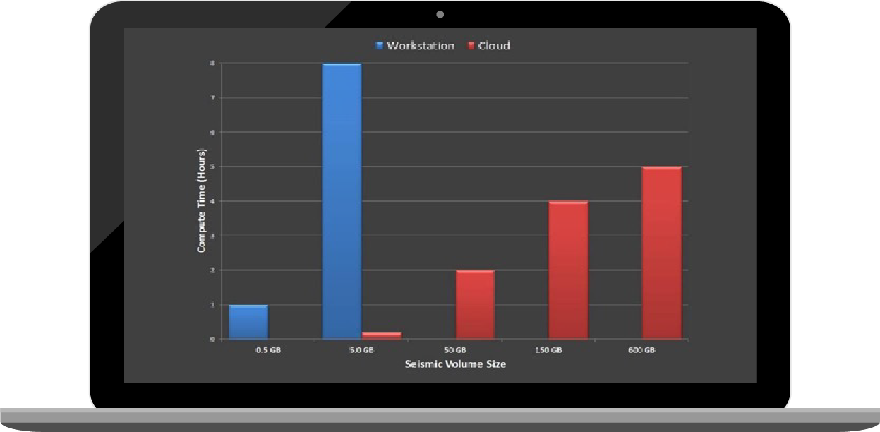
Let’s analyze some comparative data to understand this better. In Figure 1:
As evident, the Seismic Engine brings about significant time savings while also generating superior fault imaging results.
The Seismic Engine also allows us to automate many geophysical processes. For example, variations in the interpretation of faults can be simulated by exploiting the imaging differences between seismic angle stacks and varying the fault likelihood parameters. Combining these different realizations in various statistically meaningful ways allows us to quantify uncertainty and incorporate that into the prospect risk evaluation process.
With traditional physics-based fault imaging approaches, even advanced attributes such as fault likelihood have limitations. For example, these attributes typically require a clean break in the seismic data to identify a fault. However, many faults are not imaged clearly due to seismic processing limitations, thus, these approaches can have trouble in noisy data. During manual interpretation, an experienced geoscientist can often overcome these limitations by correctly identifying the faults even in poorly imaged seismic images. However, it is time-consuming and tedious work. Landmark’s machine learning approach to fault imaging incorporates elements of the interpreter’s learned knowledge into our automated workflows that deliver crisp and accurate results.
Landmark has shown that Convolutional Neural Networks (CNN) are effective tools for solving image classification problems such as identifying faults in seismic data.
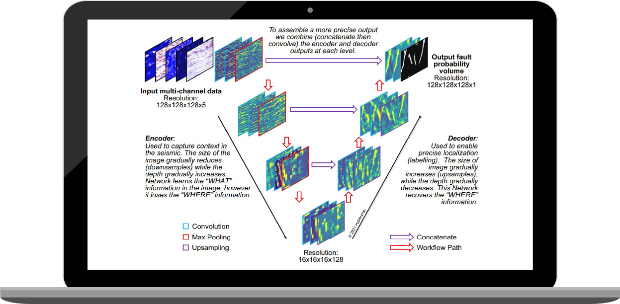
A CNN is a deep learning algorithm that can take an input image, assign importance to various aspects in the image, and then be able to differentiate one aspect from another. The algorithm does this through a series of layers each more sophisticated at identifying details in an image than the previous one. In a U-Net CNN architecture, which is essentially two mirrored CNNs, an output image of the same size as the input is generated but with specific features predicted (Figure 2). The process is to first train a model based on a subset of synthetic data with known answers (input seismic + fault labels), then run that model on the full dataset to generate a fault probability volume.
Seismic attributes can be leveraged to improve this process. We incorporate this additional information into our training and prediction process as new channels into an extended U-Net architecture. To determine which seismic attributes work best, we use a machine learning technique called a Random Forrest (RF) architecture.
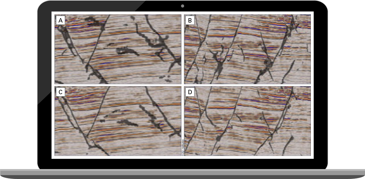
In addition to using synthetic data to train the models, real data and its manual interpretation can also be used, but you must be careful. Synthetic data allows us to create examples where there is only one possible correct interpretation. Thus, the model is always being trained with the correct answer. However, real, field-acquired seismic data and its manual (human) interpretation is not so simple. Even experienced interpreters can come up with different interpretations of the same seismic data. There isn't one correct approach to training a model. As such, examples from real datasets need to be selected with caution, preferably where the potential variation in answers is minimal. Luckily, only a small amount is needed to make a noticeable improvement in prediction accuracy (Figure 3). Landmark can augment machine learning workflows with client data to generate custom models tuned for specific geologic scenarios and challenges.
A final machine learning technique can be applied as a post-processing step to fine-tune the fault probability image. Generative Adversarial Networks (GANs) are algorithmic architectures that pit two neural networks against each other (thus the “adversarial”). One network creates new images while the other network tries to classify the images as real or fake. The two models are trained together until one outwits the other. Fault images reconstructed with GANs display clearer, thinner, and more continuous segments.
Images from: