January 30, 2023
When constructing a robust structural model to help appraise assets, confidence in the quality of input data within the interpretation package is imperative. One method of measuring data quality and consistency is the calculation of well-seismic mistie. Mistie values can give a clear insight into the consistency between a domain-converted interpretation of 2D/3D seismic data via a velocity model, and wells picked by a geoscientist. The values highlight areas that potentially need reinterpretation.
Traditional Mistie Gridding workflows are lengthy, click intensive and difficult to replicate, with the desired grid extents hard to achieve. The addition of ‘Mistie Gridding and Residual Fit’ functionality in the recent release of Geosciences Suite, a DecisionSpace® 365 solution streamlines the generation of correction and difference outputs through new user interface (UI) and visualization tools. The new Mistie Gridding algorithm helps ensure that the output results match the input data extent. Mistie Gridding has also been integrated with the ‘Zone Analysis’ tool in Velocity Modelling, allowing greater choice and refinement of data inputs.
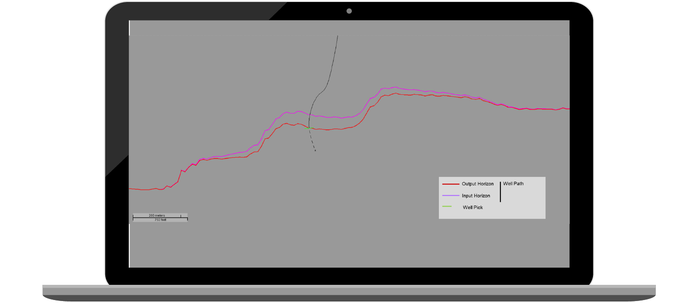
Mistie Gridding uses the radial data function ‘Thin Plate Spline’, to calculate Correction and Difference maps from depth/time seismic horizons and grids. This allows the interpretation to fit surface picks, while minimizing potential loss of data fidelity (see figure 1).
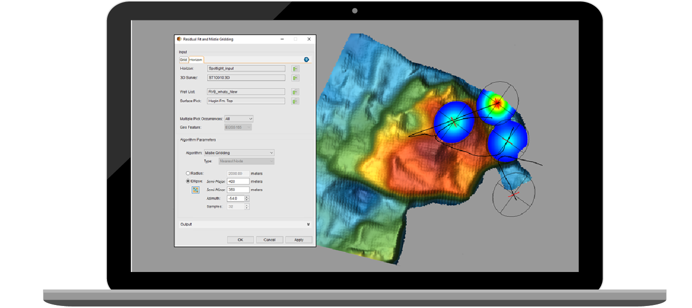
Mistie Gridding generates a correction output based upon a defined radius or ellipse, centered on surface picks, using either the Nearest Node or Interpolation methods. Outside of the defined radius or ellipse, the magnitude of correction is zero, and the output is fitted to exactly match the data input. The new ‘Mistie Gridding and Residual Fit’ UI allows the definition of ellipse major, minor axes, and azimuth inside the application. Alternatively, a new visualization tool can be used to draw and scale the ellipse definitions within the Map Editor (see Figure 2).
As shown in Figure 2, the magnitude of mistie and relationships between wells can be clearly identified and qualitatively assessed, in the context of an output grid that directly resembles the input seismic data. The resulting output Correction Map can be processed and quantitatively assessed within the ‘Zone Analysis’ tool, where data input selection can be refined, along with the calculation method.
The integration of a new dedicated Mistie Gridding UI with 'Zone Analysis' data selection functionality allows the ability to generate iterative results on the fly. This helps enable a streamlined workflow, reduce the uncertainty surrounding data inclusion, with results that are easy to analyze.